Usage: 2D

The 2D model resolves constructive systems whose section is not a simple stack of homogeneous layers: hollow blocks (HollowBlock, walls) and joist-and-block slabs (Slab, roofs). The Quickstart steps are the same as in 1D. The differences are the class (System2D), that tilt must be 90 (HollowBlock) or 0 (Slab), and that the 2D element goes inside the layer stack.

As in Usage: 1D, the examples show real results for the average day of May in Cuernavaca. Building the systems and inspecting their sections is executed live when this documentation is rendered. The solves are pre-computed by docs/run_examples.py, because a default-mesh 2D solve takes about 25 minutes in a modern CPU; this page reads and plots its outputs (in docs/data/results/).

2D geometries

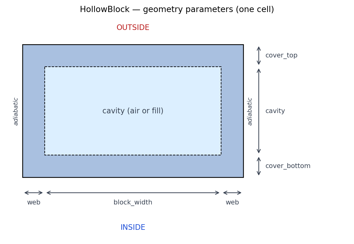
The 2D elements (HollowBlock for walls, Slab for joist-and-block roofs) are defined by a geometry dictionary, with measures in metres. The schemes below name every key, drawn to scale with the same values used in the examples further down (shown in mm for readability):

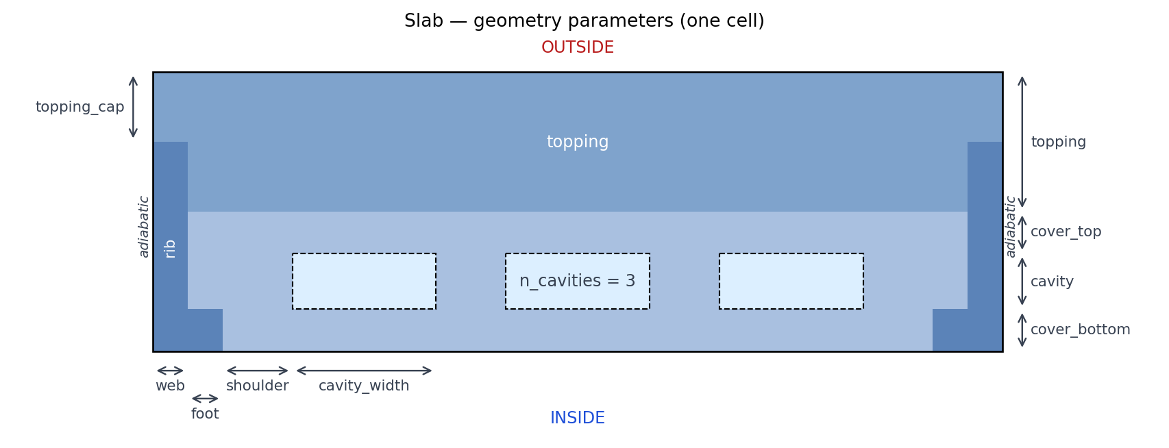
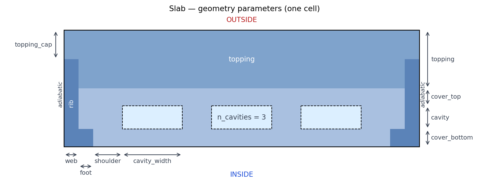
The rib is an L: its web rises through the whole element (stopping below the full-width topping_cap) and its foot widens it only along the cover_bottom band, forming the ledge the filler block rests on.

The OUTSIDE face exchanges heat with the sun–air temperature and the INSIDE face with the indoor air; the lateral cuts are adiabatic symmetry planes of the repeating pattern. The boundary conditions are stated, with their domain figure, in the 2D model.

Examples

Free-running and air-conditioned, for a hollow-block wall and a joist-and-block roof. Setup shared by all the examples (the materials are defined in the materials file):

import enerhabitat as eh
import pandas as pd
import matplotlib.pyplot as plt   # Comment or delete if not creating visualization
import matplotlib.dates as mdates # Comment or delete if not creating visualization


eh.config.file = "data/materials.ini"
epw_file = "data/MEX_MOR_Cuernavaca-Matamoros.Intl.AP.767260_TMYx.2004-2018.epw"

Plot helper used by the examples (click to show)

EH_COLORS = {"Ti": "#2a78d6", "Tsa": "#eb6834", "Ta": "#008300", "Tn": "#6b7280"}

def plot_day(df, title=""):
    """Temperatures of the average day (with the comfort zone Tn ± DeltaTn)
    and the solar irradiance components carried by the same dataframe."""
    fig, (ax, axr) = plt.subplots(2, 1, figsize=(7.2, 5.8), sharex=True,
                                  height_ratios=[3, 2])

    # --- temperatures ---
    # comfort zone: Tn and DeltaTn are columns (constant along the day)
    ax.fill_between(df.index, df["Tn"] - df["DeltaTn"], df["Tn"] + df["DeltaTn"],
                    color=EH_COLORS["Tn"], alpha=0.12, lw=0)
    ax.plot(df["Tn"], color=EH_COLORS["Tn"], ls="--", lw=1, label="Tn ± ΔTn")

    ax.plot(df["Ta"],  color=EH_COLORS["Ta"],  lw=2, label="Ta")
    ax.plot(df["Tsa"], color=EH_COLORS["Tsa"], lw=2, label="Tsa")
    ax.plot(df["Ti"],  color=EH_COLORS["Ti"],  lw=2, label="Ti")

    ax.set_ylabel("temperature (°C)")
    ax.set_title(title, fontsize=10)
    ax.legend(frameon=False, fontsize=9, loc="upper left")

    # --- solar irradiance (same dataframe: Ig, Ib, Id from the EPW; Is on the
    # tilted/oriented surface, computed by Tsa()) ---
    axr.plot(df["Ig"], color="#f59e0b", lw=1.5, label="Ig (global horizontal)")
    axr.plot(df["Ib"], color="#a16207", lw=1.5, label="Ib (direct normal)")
    axr.plot(df["Id"], color="#60a5fa", lw=1.5, label="Id (diffuse horizontal)")
    axr.plot(df["Is"], color="#dc2626", lw=2,   label="Is (on the surface)")

    axr.set_ylabel("irradiance (W/m²)")
    axr.set_xlabel("hour of the average day (civil time)")
    axr.legend(frameon=False, fontsize=8, loc="upper left")

    # tz=... keeps the labels in local time (matplotlib defaults to UTC)
    axr.xaxis.set_major_locator(mdates.HourLocator(byhour=[0, 6, 12, 18], tz=df.index.tz))
    axr.xaxis.set_major_formatter(mdates.DateFormatter("%H", tz=df.index.tz))

    for a in (ax, axr):
        a.grid(alpha=0.25, lw=0.5)
        a.spines["top"].set_visible(False)
        a.spines["right"].set_visible(False)
    fig.tight_layout()
    plt.show()

2D hollow-block wall, free-running

A concrete block with one air cavity per cell. The 2D element goes inside the layer stack; finishes are ordinary 1D layers around it. Building the system is instantaneous (only solve() is expensive):

block = eh.HollowBlock(
    material   = "Concreto",          # single material of the block
    emissivity = 0.9,                 # cavity-wall emissivity (radiation)
    geometry   = {                    # cell measures, in metres
        "web":          0.02,         # half web (rib) thickness
        "block_width":  0.16,         # cavity width
        "cover_top":    0.02,         # outer shell
        "cavity":       0.08,         # cavity height
        "cover_bottom": 0.02,         # inner shell
    },
)

wall2d = eh.System2D(eh.Location(epw_file))
wall2d.tilt = 90                      # walls only (required for HollowBlock)
wall2d.azimuth = 90
wall2d.absortance = 0.6
wall2d.layers = [("Mortero", 0.02), block, ("Yeso", 0.01)]
# 2D stacks accept at most 7 layers INCLUDING the 2D element (fixed slots
# inherited from the C engine); exceeding it raises ValueError. 1D has no limit.

The section scheme, to scale, with the outside on top. This is one of several ways to check the geometry before solving: preview() can also draw the node types and the k and ρc fields, section_report() prints a verification table, and there is an ASCII backend for terminals, all demonstrated in Inspecting the section:

wall2d.preview(field="materials");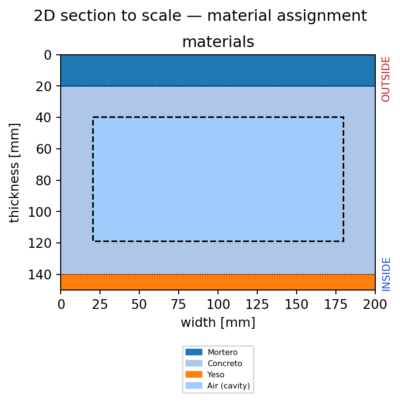

import numpy as np   # Required to visualize temperature field, comment if not needed
import json   # Required to save results and be read again later


wall2d.location.meanDay(month=5, year=2025)
wall2d.Tsa()

ti = wall2d.solve()                   # free-running — ~25 min (default mesh)

# Look at the results before saving them:
print(wall2d.energy_transfer)         # J/(m²·day), per unit indoor area
print(wall2d.days)                    # days iterated to reach the periodic regime

# A 2D solve is expensive: SAVE the results, so you pay that time only once.
# Ti and the surface/cavity Series concatenate with Tsa(), as in the 1D;
# Tfield is the (nx, ny) °C field of the last (converged) day.
data = pd.concat([ti, wall2d.Tso, wall2d.Tsi, wall2d.Thueco, wall2d.Tsa()], axis=1)
data.to_csv("data/results/hollow_free.csv")
np.save("data/results/hollow_free_Tfield.npy", wall2d.Tfield)

# The scalar results are attributes, not columns of the CSV: keep them too.
scalars = {"energy_transfer": wall2d.energy_transfer, "days": wall2d.days}
json.dump(scalars, open("data/results/hollow_free_scalars.json", "w"))

Reading the stored files back follows the same workflow: same columns, same plots, no re-solving. That is exactly what this page does; its files were written by docs/run_examples.py with the code above, with one difference of bookkeeping: instead of one JSON per case, it gathers the scalars of the three cases (energies, convergence days, runtime, and the mesh extent in mm that the Tfield plots need) into a single data/results/summary.json, which the cells below read:

# The 2D results were computed and saved beforehand by docs/run_examples.py;
# json reads the stored summary (energies, convergence days, runtimes).
import json

RES = "data/results"
summary = json.load(open(f"{RES}/summary.json"))

hollow = pd.read_csv(f"{RES}/hollow_free.csv", index_col=0, parse_dates=True)
s = summary["hollow_free"]
print(f"energy_transfer = {s['energy_transfer']:,.1f} J/(m²·day)"
      f"  = {s['energy_transfer']/3600:,.1f} Wh/(m²·day)"
      f"  ·  converged in {s['days']} days")
plot_day(hollow, title="Hollow-block wall (2D), east, free-running — May, Cuernavaca")

energy_transfer = 47,610.0 J/(m²·day)  = 13.2 Wh/(m²·day)  ·  converged in 4 days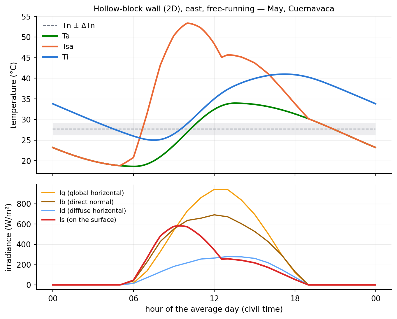

Besides Ti, the 2D solver keeps the full temperature field of the last (converged) day: wall2d.Tfield, an (nx, ny) array in °C on the section mesh, with the same orientation as preview() (outside on top):

import numpy as np

T = np.load(f"{RES}/hollow_free_Tfield.npy")
s = summary["hollow_free"]
fig, ax = plt.subplots(figsize=(7.0, 3.8))
im = ax.imshow(T.T, extent=[0, s["X_mm"], s["Y_mm"], 0], aspect="equal",
               cmap="inferno", interpolation="nearest")
fig.colorbar(im, ax=ax, label="T (°C)")
ax.set_xlabel("width [mm]")
ax.set_ylabel("thickness [mm]")
ax.set_title("Tfield — hollow-block wall, end of the converged day", fontsize=10)
fig.tight_layout()
plt.show()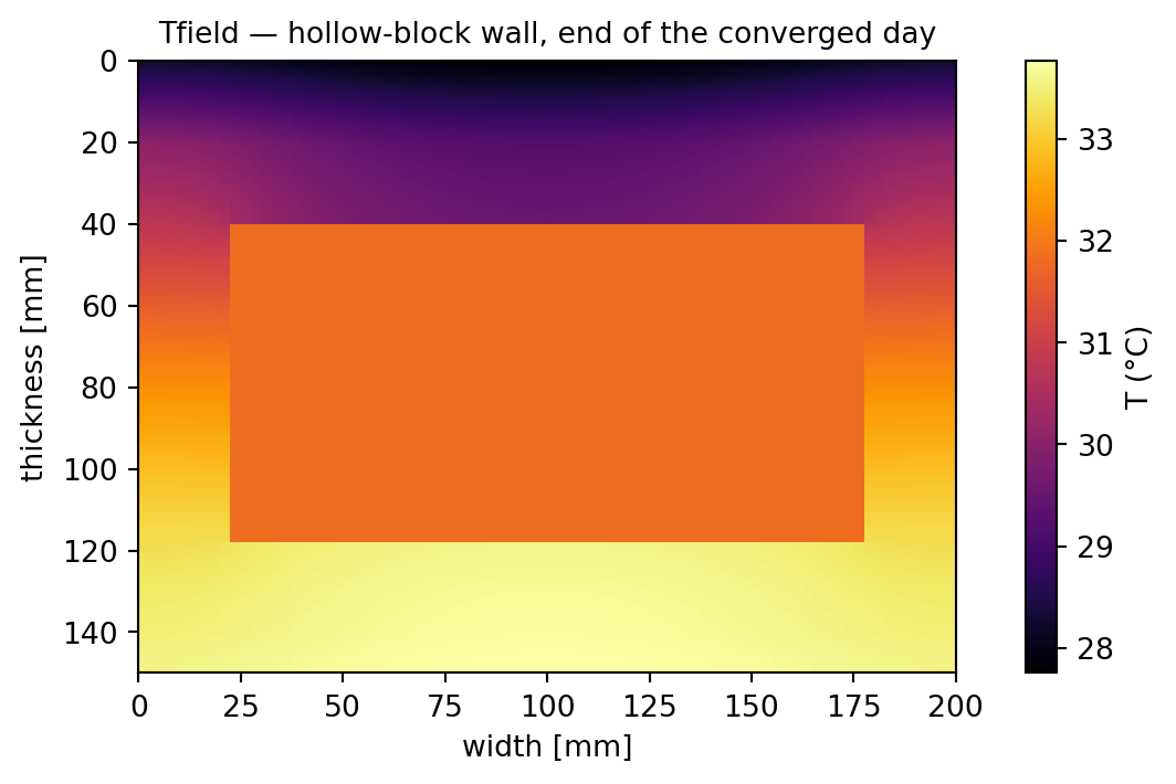

2D hollow-block wall, air-conditioned

tiAC = wall2d.solveAC()               # Ti held at Tn
print(wall2d.cooling_energy, wall2d.heating_energy)

pd.concat([tiAC, wall2d.Tso, wall2d.Tsi, wall2d.Thueco, wall2d.Tsa()],
          axis=1).to_csv("data/results/hollow_ac.csv")   # save, as before

hollowAC = pd.read_csv(f"{RES}/hollow_ac.csv", index_col=0, parse_dates=True)
s = summary["hollow_ac"]
print(f"cooling_energy = {s['cooling_energy']:,.0f} J/(m²·day)"
      f"  = {s['cooling_energy']/3600:,.1f} Wh/(m²·day)")
print(f"heating_energy = {s['heating_energy']:,.0f} J/(m²·day)"
      f"  = {s['heating_energy']/3600:,.1f} Wh/(m²·day)")
plot_day(hollowAC, title="Hollow-block wall (2D), air-conditioned — May, Cuernavaca")

cooling_energy = 1,574,884 J/(m²·day)  = 437.5 Wh/(m²·day)
heating_energy = 287,568 J/(m²·day)  = 79.9 Wh/(m²·day)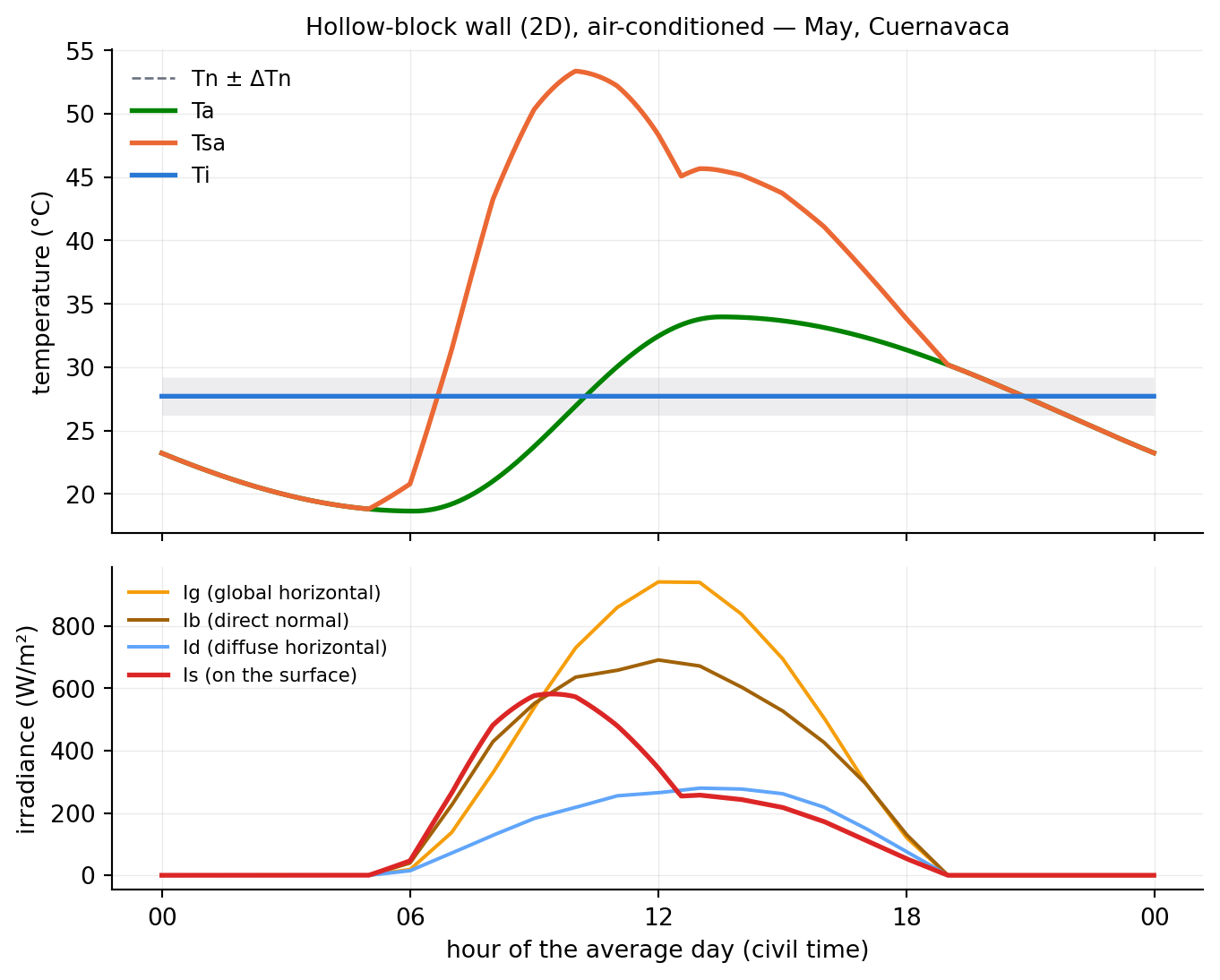

Joist-and-block roof (`Slab`)

Three solids (compression topping, L-shaped rib, filler block) plus N equal cavities that can be air (Fill.AIR) or a solid fill (Fill.SOLID).

slab = eh.Slab(
    rib_material     = "ConcretoAltaDensidad",   # joist/rib (L-shaped: web + foot)
    block_material   = "Bovedilla",              # filler block around the cavities
    topping_material = "Concreto",               # compression topping
    fill_type        = eh.Fill.AIR,      # or eh.Fill.SOLID (+ fill_material)
    emissivity       = 0.9,              # required if AIR
    geometry = {
        "web":          0.025,   # rib web
        "foot":         0.025,   # rib foot
        "shoulder":     0.050,   # block between rib and cavities
        "n_cavities":   3,
        "cavity_width": 0.103,
        "topping":      0.100,   # compression topping
        "topping_cap":  0.050,   # topping above the rib web
        "cover_top":    0.030,   # block above the cavity
        "cavity":       0.040,   # cavity height
        "cover_bottom": 0.030,   # block below the cavity
    },
)

roof = eh.System2D(eh.Location(epw_file))
roof.tilt = 0                            # roofs only (required for Slab)
roof.absortance = 0.3
roof.layers = [("Impermeabilizante", 0.003), slab, ("Yeso", 0.015)]

roof.preview(field="materials");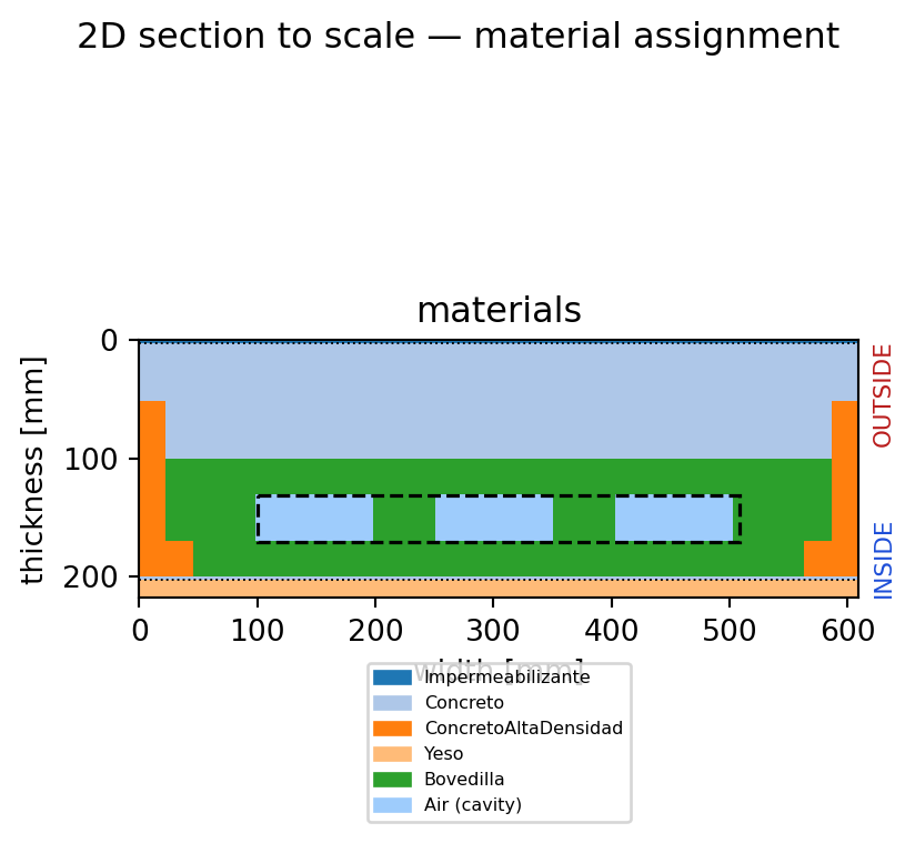

roof.location.meanDay(month=5, year=2025)
roof.Tsa()

ti = roof.solve()                        # or roof.solveAC()

print(roof.energy_transfer)              # J/(m²·day)
print(roof.days)                         # days to the periodic regime

# Same recommendation as with the wall: save, then analyse from the files.
data = pd.concat([ti, roof.Tso, roof.Tsi, roof.Thueco, roof.Tsa()], axis=1)
data.to_csv("data/results/slab_free.csv")
np.save("data/results/slab_free_Tfield.npy", roof.Tfield)

Recovered from the stored files:

slab_df = pd.read_csv(f"{RES}/slab_free.csv", index_col=0, parse_dates=True)
s = summary["slab_free"]
print(f"energy_transfer = {s['energy_transfer']:,.0f} J/(m²·day)"
      f"  = {s['energy_transfer']/3600:,.1f} Wh/(m²·day)"
      f"  ·  converged in {s['days']} days")
plot_day(slab_df, title="Joist-and-block roof (2D), free-running — May, Cuernavaca")

energy_transfer = 26,545 J/(m²·day)  = 7.4 Wh/(m²·day)  ·  converged in 6 days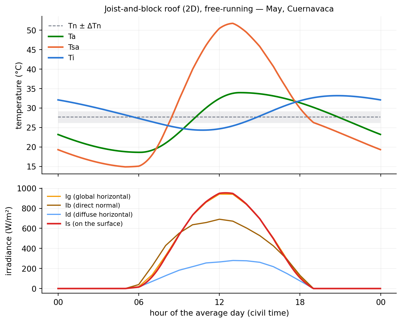

Note how the roof’s Tsa drops below Ta at night: that is the long-wave radiation factor (\(RF = 3.9\) °C for horizontal surfaces) at work. The roof sees the cold sky (see the 1D model).

The 2D results go beyond Ti: the read-only Series Tso (outdoor surface), Tsi (indoor surface) and Thueco (cavity air) live on the same time grid, plotted here alongside Ti:

fig, ax = plt.subplots(figsize=(7.2, 3.6))
ax.plot(slab_df["Tso"],    color="#eb6834", lw=2, label="Tso (outdoor surface)")
ax.plot(slab_df["Thueco"], color="#9467bd", lw=2, label="Thueco (cavity air)")
ax.plot(slab_df["Tsi"],    color="#0d9488", lw=2, label="Tsi (indoor surface)")
ax.plot(slab_df["Ti"],     color="#2a78d6", lw=2, label="Ti (indoor air)")
ax.xaxis.set_major_locator(mdates.HourLocator(byhour=[0, 6, 12, 18], tz=slab_df.index.tz))
ax.xaxis.set_major_formatter(mdates.DateFormatter("%H", tz=slab_df.index.tz))
ax.set_xlabel("hour of the average day")
ax.set_ylabel("temperature (°C)")
ax.set_title("Roof surfaces: the cavity damps the outdoor swing", fontsize=10)
ax.legend(frameon=False, fontsize=9, loc="upper left")
ax.grid(alpha=0.25, lw=0.5)
ax.spines["top"].set_visible(False)
ax.spines["right"].set_visible(False)
fig.tight_layout()
plt.show()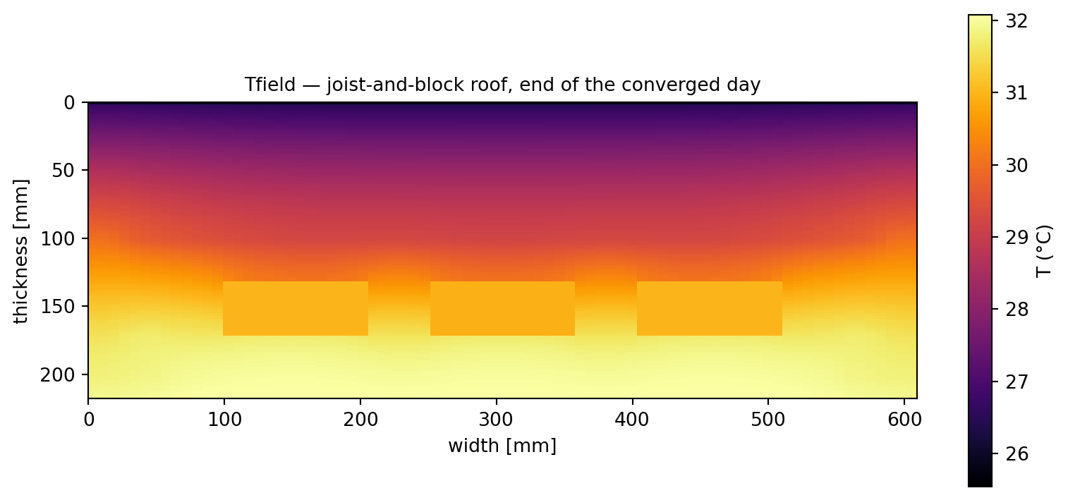

And its temperature field, where the joists show up as thermal bridges through the cavity band:

T = np.load(f"{RES}/slab_free_Tfield.npy")
s = summary["slab_free"]
fig, ax = plt.subplots(figsize=(8.5, 3.8))
im = ax.imshow(T.T, extent=[0, s["X_mm"], s["Y_mm"], 0], aspect="equal",
               cmap="inferno", interpolation="nearest")
fig.colorbar(im, ax=ax, label="T (°C)")
ax.set_xlabel("width [mm]")
ax.set_ylabel("thickness [mm]")
ax.set_title("Tfield — joist-and-block roof, end of the converged day", fontsize=10)
fig.tight_layout()
plt.show()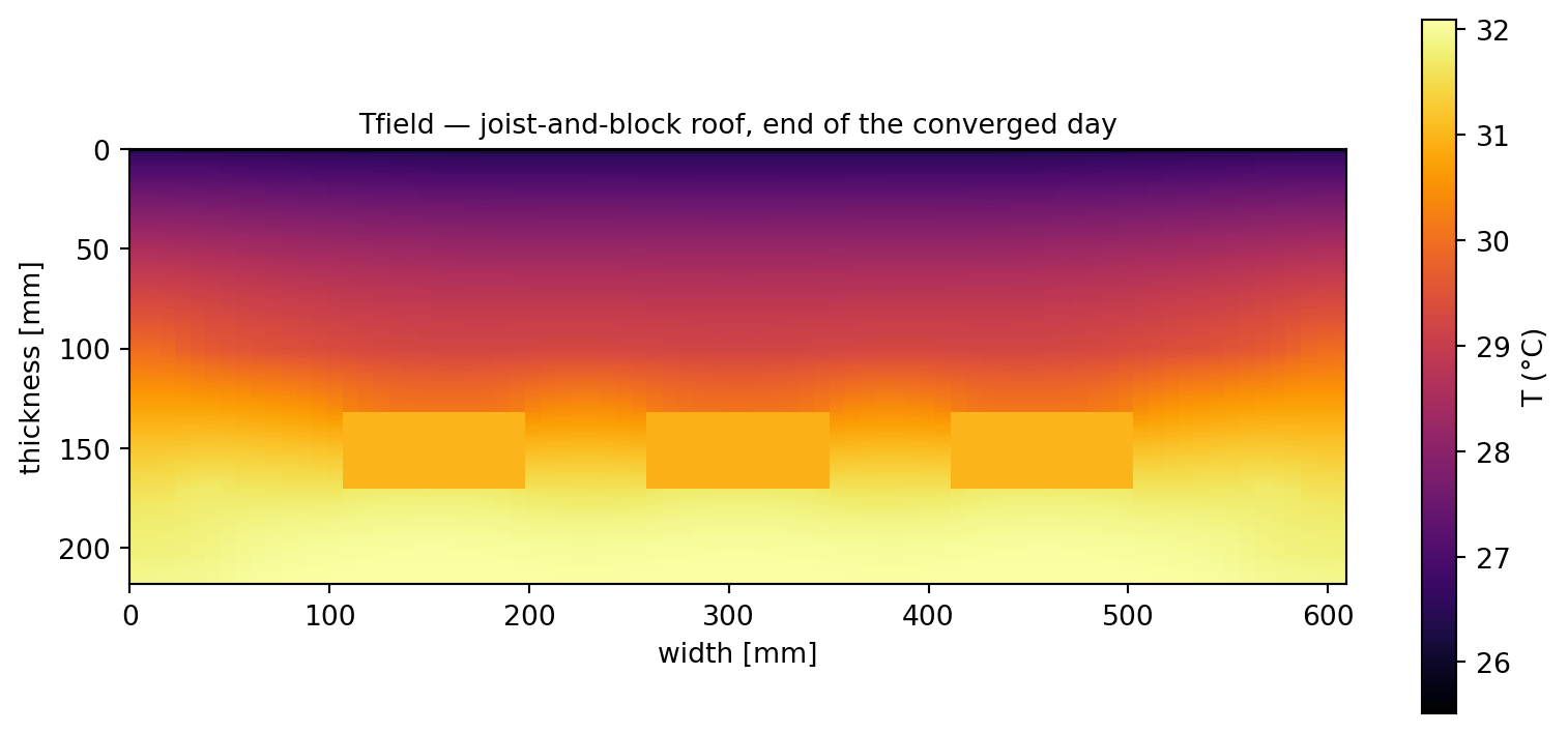

Filled cavities (`Fill.SOLID`)

The cavity of a HollowBlock (or the cavities of a Slab) can be filled with a solid material instead of air, e.g. an insulating core:

block = eh.HollowBlock(
    material      = "Concreto",
    fill_type     = eh.Fill.SOLID,
    fill_material = "EPS",
    geometry      = {"web": 0.02, "block_width": 0.16,
                     "cover_top": 0.02, "cavity": 0.08, "cover_bottom": 0.02},
)

Filling with the same material as the shell makes the unit homogeneous, equivalent to a 1D layer (this is one of the package’s validation checks).

Inspecting the section

Before solving you can inspect, to scale, how materials and node types are laid out on the 2D mesh. The section schemes shown with each example above were drawn by preview(field="materials"). section_report() prints the verification table:

wall2d.section_report()            # table: node types + materials (k, ρc, y-range)

2D section  80×160   X=200.0 mm  Y=150.0 mm   dx=2.500  dy=0.938 mm
Block/cavity: i∈[8,72)  j∈[42,127)
Node types (NT):
    NT  0  air             5440 nodes
    NT  1  corner             1 nodes
    NT  2  corner             1 nodes
    NT  3  corner             1 nodes
    NT  4  corner             1 nodes
    NT  5  outer edge        78 nodes
    NT  6  side             158 nodes
    NT  7  side             158 nodes
    NT  8  inner edge        78 nodes
    NT  9  top wall          64 nodes
    NT 10  bottom wall       64 nodes
    NT 11  left wall         85 nodes
    NT 12  right wall        85 nodes
    NT 13  interior        6586 nodes
Assigned materials (by k, ρc):
    Mortero                        1760 nodes   y∈[0.0,20.6] mm  (k=0.7, ρc=1.8e+06)
    Concreto                       4800 nodes   y∈[20.6,140.6] mm  (k=1.8, ρc=1.936e+06)
    Yeso                            800 nodes   y∈[140.6,150.0] mm  (k=0.37, ρc=900000)
    Air (cavity)                   5440 nodes   y∈[39.4,119.1] mm

The default preview() draws three panels: the node types (the finite-volume classification each mesh node gets: interior, cavity walls, corners, air), and the k and ρc fields actually assigned to the mesh:

wall2d.preview();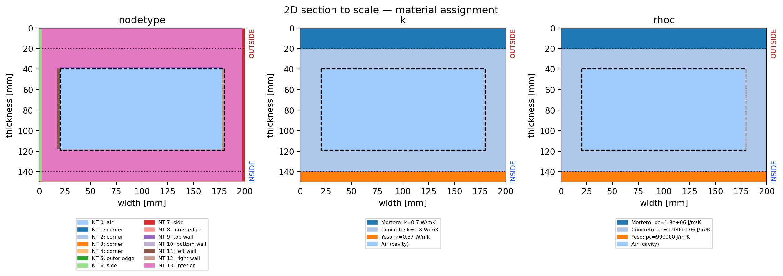

matplotlib is an optional extra (pip install enerhabitat[viz]). Without it, or with backend="ascii", the inspector falls back to a to-scale ASCII drawing, handy on a remote terminal. Note that the drawing is a resampling of the mesh, not the mesh itself: one character is not one node. Each character shows the node nearest to its position, and the header states the resolution (chars vs. mesh nodes, and the size in mm each character covers):

roof.preview(field="materials", backend="ascii")

  [materials]  to-scale cut  X=609mm × Y=218mm (outside on top)
  60×11 chars resampled from the 80×160 mesh (1 char ≈ 10.2×19.8 mm, nearest node)
  ▓▓▓▓▓▓▓▓▓▓▓▓▓▓▓▓▓▓▓▓▓▓▓▓▓▓▓▓▓▓▓▓▓▓▓▓▓▓▓▓▓▓▓▓▓▓▓▓▓▓▓▓▓▓▓▓▓▓▓▓   ← OUTSIDE
  ▓▓▓▓▓▓▓▓▓▓▓▓▓▓▓▓▓▓▓▓▓▓▓▓▓▓▓▓▓▓▓▓▓▓▓▓▓▓▓▓▓▓▓▓▓▓▓▓▓▓▓▓▓▓▓▓▓▓▓▓
  ▓▓▓▓▓▓▓▓▓▓▓▓▓▓▓▓▓▓▓▓▓▓▓▓▓▓▓▓▓▓▓▓▓▓▓▓▓▓▓▓▓▓▓▓▓▓▓▓▓▓▓▓▓▓▓▓▓▓▓▓
  ▒▒▓▓▓▓▓▓▓▓▓▓▓▓▓▓▓▓▓▓▓▓▓▓▓▓▓▓▓▓▓▓▓▓▓▓▓▓▓▓▓▓▓▓▓▓▓▓▓▓▓▓▓▓▓▓▓▓▒▒
  ▒▒▓▓▓▓▓▓▓▓▓▓▓▓▓▓▓▓▓▓▓▓▓▓▓▓▓▓▓▓▓▓▓▓▓▓▓▓▓▓▓▓▓▓▓▓▓▓▓▓▓▓▓▓▓▓▓▓▒▒
  ▒▒++++++++++++++++++++++++++++++++++++++++++++++++++++++++▒▒
  ▒▒++++++++++++++++++++++++++++++++++++++++++++++++++++++++▒▒
  ▒▒++++++++··········+++++··········+++++··········++++++++▒▒
  ▒▒++++++++··········+++++··········+++++··········++++++++▒▒
  ▒▒▒▒▒++++++++++++++++++++++++++++++++++++++++++++++++++▒▒▒▒▒
  ░░░░░░░░░░░░░░░░░░░░░░░░░░░░░░░░░░░░░░░░░░░░░░░░░░░░░░░░░░░░   ← INSIDE
  legend:
    '█'  Impermeabilizante
    '▓'  Concreto
    '▒'  ConcretoAltaDensidad
    '░'  Yeso
    '+'  Bovedilla
    '·'  Air (cavity)

The raw arrays are also available: sec = wall2d.section() returns the node-type, k and ρc fields together with the mesh.

The 2D mesh and convergence parameters (nx, ny, tolerances, iteration caps) live in config2d, documented with the rest of the configuration in Usage — setup.