Usage: 1D

The Quickstart steps applied to a homogeneous layer stack, in both modes, free-running and air-conditioned. The examples show real results for the average day of May in Cuernavaca, Mexico (the EPW and materials.ini used here live in docs/data/ in the repository), and are executed when this documentation is rendered.

Setup shared by all the examples:

import enerhabitat as eh
import pandas as pd
import matplotlib.pyplot as plt   # Comment or delete if not creating visualization
import matplotlib.dates as mdates # Comment or delete if not creating visualization


eh.config.file = "data/materials.ini"
epw_file = "data/MEX_MOR_Cuernavaca-Matamoros.Intl.AP.767260_TMYx.2004-2018.epw"

Plot helper used by the examples (click to show)

EH_COLORS = {"Ti": "#2a78d6", "Tsa": "#eb6834", "Ta": "#008300", "Tn": "#6b7280"}

def plot_day(df, title=""):
    """Temperatures of the average day (with the comfort zone Tn ± DeltaTn)
    and the solar irradiance components carried by the same dataframe."""
    fig, (ax, axr) = plt.subplots(2, 1, figsize=(7.2, 5.8), sharex=True,
                                  height_ratios=[3, 2])

    # --- temperatures ---
    # comfort zone: Tn and DeltaTn are columns (constant along the day)
    ax.fill_between(df.index, df["Tn"] - df["DeltaTn"], df["Tn"] + df["DeltaTn"],
                    color=EH_COLORS["Tn"], alpha=0.12, lw=0)
    ax.plot(df["Tn"], color=EH_COLORS["Tn"], ls="--", lw=1, label="Tn ± ΔTn")

    ax.plot(df["Ta"],  color=EH_COLORS["Ta"],  lw=2, label="Ta")
    ax.plot(df["Tsa"], color=EH_COLORS["Tsa"], lw=2, label="Tsa")
    ax.plot(df["Ti"],  color=EH_COLORS["Ti"],  lw=2, label="Ti")

    ax.set_ylabel("temperature (°C)")
    ax.set_title(title, fontsize=10)
    ax.legend(frameon=False, fontsize=9, loc="upper left")

    # --- solar irradiance (same dataframe: Ig, Ib, Id from the EPW; Is on the
    # tilted/oriented surface, computed by Tsa()) ---
    axr.plot(df["Ig"], color="#f59e0b", lw=1.5, label="Ig (global horizontal)")
    axr.plot(df["Ib"], color="#a16207", lw=1.5, label="Ib (direct normal)")
    axr.plot(df["Id"], color="#60a5fa", lw=1.5, label="Id (diffuse horizontal)")
    axr.plot(df["Is"], color="#dc2626", lw=2,   label="Is (on the surface)")

    axr.set_ylabel("irradiance (W/m²)")
    axr.set_xlabel("hour of the average day (civil time)")
    axr.legend(frameon=False, fontsize=8, loc="upper left")

    # tz=... keeps the labels in local time (matplotlib defaults to UTC)
    axr.xaxis.set_major_locator(mdates.HourLocator(byhour=[0, 6, 12, 18], tz=df.index.tz))
    axr.xaxis.set_major_formatter(mdates.DateFormatter("%H", tz=df.index.tz))

    for a in (ax, axr):
        a.grid(alpha=0.25, lw=0.5)
        a.spines["top"].set_visible(False)
        a.spines["right"].set_visible(False)
    fig.tight_layout()
    plt.show()

1D wall, free-running

wall = eh.System(eh.Location(epw_file))
wall.azimuth = 90                    # east-facing
wall.absortance = 0.3
wall.layers = [("Mortero", 0.025), ("Ladrillo", 0.10)]
wall.location.meanDay(month=5, year=2025)
wall.Tsa()

data = wall.solve()                  # free-running Ti
data = pd.concat([data, wall.Tso, wall.Tsi, wall.Tsa()], axis=1)

print(f"energy_transfer = {wall.energy_transfer:,.0f} J/(m²·day)"
      f"  = {wall.energy_transfer/3600:,.1f} Wh/(m²·day)")

energy_transfer = 31,973 J/(m²·day)  = 8.9 Wh/(m²·day)

Both solvers return a pandas.Series named "Ti", indexed by time of day on the same time grid as Tsa(); that is why the pd.concat above aligns without NaN and promotes the Series to a column. The surface temperatures of the last solve are available the same way, as the read-only Series wall.Tso (outdoor surface) and wall.Tsi (indoor surface). When a DataFrame is required, convert with wall.solve().to_frame("Ti").

plot_day(data, title="Mortero + Ladrillo wall, east, free-running — May, Cuernavaca")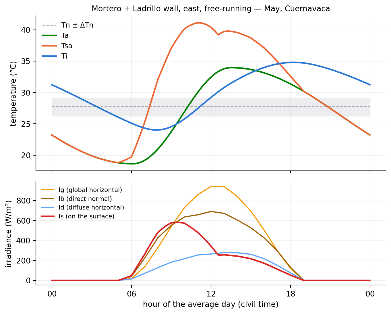

The time axis is civil (clock) time, inherited from the EPW, not solar time. That is why this east-facing wall keeps direct sun past 12:00: solar noon in Cuernavaca falls at about 12:33 (the site lies 9.2° west of the UTC−6 reference meridian, which adds 37 min, minus some 4 min of equation of time in May). The sharp drop in Is (mirrored by Tsa) marks that moment: the sun crosses due south and the east wall is left with diffuse irradiance only.

1D wall, air-conditioned

Same wall; solveAC() holds Ti at the neutrality temperature Tn and reports the energy needed to do so:

dataAC = wall.solveAC()
dataAC = pd.concat([dataAC, wall.Tsa()], axis=1)

print(f"cooling_energy = {wall.cooling_energy:,.0f} J/(m²·day)"
      f"  = {wall.cooling_energy/3600:,.1f} Wh/(m²·day)")
print(f"heating_energy = {wall.heating_energy:,.0f} J/(m²·day)"
      f"  = {wall.heating_energy/3600:,.1f} Wh/(m²·day)")

cooling_energy = 943,968 J/(m²·day)  = 262.2 Wh/(m²·day)
heating_energy = 386,936 J/(m²·day)  = 107.5 Wh/(m²·day)

plot_day(dataAC, title="Same wall, air-conditioned (Ti = Tn) — May, Cuernavaca")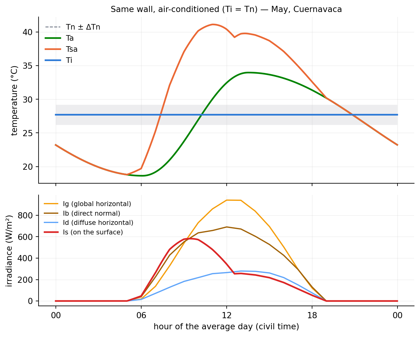

Where to go next

For systems whose section is not a simple layer stack (hollow blocks, joist-and-block slabs), continue with Usage — 2D. The global parameters (La, ho, hi, Nx) are documented in the configuration.